Introduction
Part
I: Seismic wave propagation and data acquisition 3I-1.
Seismic wave propagation
I-2. Data acquisition
Part II: Seismic processing
II-1.
CMP gather
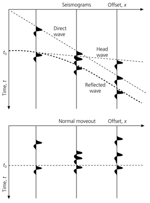
II-2. Normal Move Out correction (NMO)
II-3. Migration |
II-4
CMP stack (summed trace)
II-5. Deconvolution
II-6. Statics correction
II-7. Bandpass filter
II-8. Gain -
Conclusion |
INTRODUCTION
The
objective is to improve the signal to noise ratio. The data treatment
consists of many processing steps on the seismic trace so as to
exclude unwanted signals (noise, multiples, etc...).
Figure 1: Sparker section from the Strataforme cruise
(Stsp045). Section A. is the raw seismic data. Section B shows
the same thing after processing (G. Jouet, 2003).
|
Figure
1 shows the necessity of the seismic processing. It compares two
seismic sections, the first is raw data obtained by seismic acquisition
and the second is the same after processing.
In a
first part we introduce the subject, discuss data acquisition and
the seismic wave propagation and then we discuss seismic processing.
PART I: SEISMIC WAVE PROPAGATION AND DATA
ACQUISITION
I-1.
Seismic wave propagation
The wave paths followed can be categorized as.
The
phenomenon is more complicated due to multiple reflections:
- The peg-leg is a resonance phenomenon resulting due to a geological
source.
- First multiple: Energy is reflected at the geological interface.
- Ghost: The energy given off by the source propagates towards the
ocean surface, and then gets reflected. Thus, there is a late wave
which creates a signal deformation.
- Diffraction: The wave is scattered in all directions when it meets
a discontinuity.
PART II: SEISMIC PROCESSING
Seismic processing can be done with many software such as SITHERE,
SISBISE, SPW etc… But, in this part, we discuss the different
steps involved in the processing.The processing is divided into
two parts:§ Data reduction
- Raw seismic trace gather (CMP gather)
- Normal Move Out correction (Might also use Dip move out to further
enhance)
- CMP stack or summed trace (reflection for a single reflector is
enhanced)
- Steps repeated for all points to get§ Data Enhancement
- Statics correction
- Deconvolution (removing source signature)
- Bandpass filter (Getting rid of noise outside frequency band)
- Mute, Gain recovery
Migration
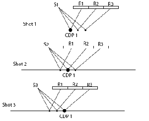
II-1. CMP gather
Reflection data transmitted from the same point (reflector) is collected
by each of the hydrophones.
Figure 4: Pattern shows the trace gather
for the first CDP. It’s the same for the other CDP. |
II-3.
Migration
Reflection
data is corrected for travel time and position relative to shot
points which can arise due to geologic structures such as synclines
and is seen as a bow tie on the stacked time series data. Migration
is an inverse wave scattering calculation that relocates seismic
reflections and diffractions to the location of their origin. Various
methods of migration are DMO and frequency domain, ray trace and
wave equation migration.
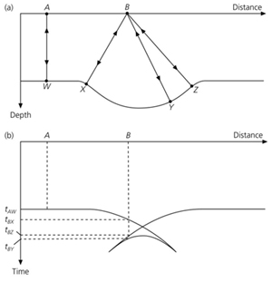
Figure 6: Migration representation. A: Real sea floor
topology with wave paths. B: Sea floor representing on a seismic
section. |
Figure 7: Seismic section example before
(a) and after (b) migration. |
II-5. Deconvolution
Seismic trace is basically a convolution of source function and
earths response. So we can use deconvolution to remove the source
signature which is known. But this isn’t as easy as it sounds
and if successful, each seismic trace is transformed into a time
series of impulses/spikes with arrival times that represent primary
reflection times to the reflectors, and amplitudes that represent
the reflection coefficients of the reflectors.
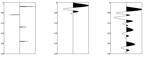
Figure
9: First: reflection signal, then: source signal, and
convolved signal |
II-7. Bandpass filter
A frequency filter allows the exclusion of noise corresponding to
lower and higher frequencies i.e. data which lies outside the reflected
frequency domain.
Figure 11: Frequency filtration pattern. |
II-8.
Gain application
Attenuation due to the head-on wave propagation results in a wave
amplitude loss which is inversely proportional to ‘r’
(wave distance covered)
Wave attenuation = higher frequency absorption. = ratio reflection/transmitting
of the wave.
The
noise amplitude increases with the signal as we go deep.
Figure 12: It shows a trace without the gain (a)
and the same trace after the correction. |
CONCLUSION
Correct processing of raw seismic data is very important as it allows
the correct interpretation of the seismic section under study.
|